This tutorial provides a brief introduction to the principles of Optical Coherence Tomography (OCT). It covers the basic theory, an introduction to Fourier domain OCT, and the difference between swept-source OCT (SS-OCT) and spectral domain OCT (SD-OCT). It also defines the key parameters for OCT systems, providing useful equations for calculating resolution, imaging depth, and sensitivity with depth, as well as discussing performance parameters like signal to noise ratio (SNR) and speed.
What is OCT?
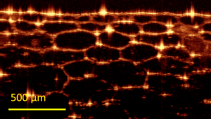
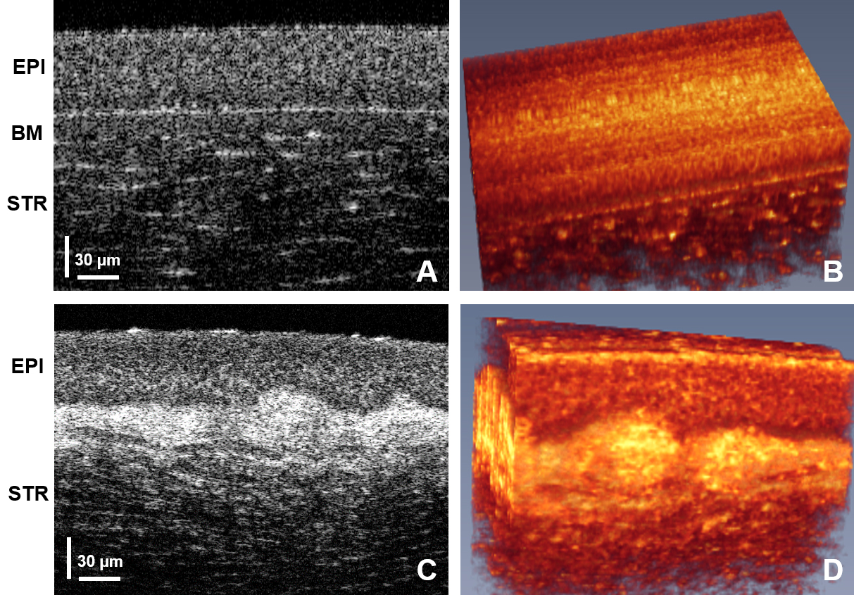
Optical coherence tomography (OCT) is a 3-D imaging technique that can provide high resolution imaging in a scattering media, non-destructively and without the need for contact or a coupling medium. Lateral imaging resolution on the order of a few micrometers is possible, to depths up to few millimeters. 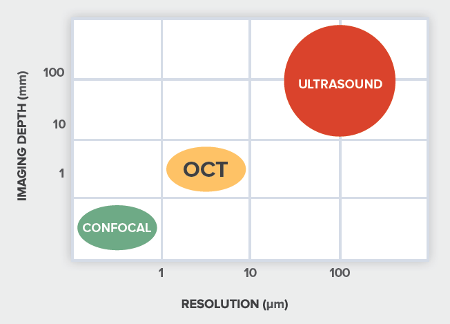 OCT’s ability to provide surface profiles and information about subsurface structure and uniformity enables it to deliver accurate information in real time for diagnostics, monitoring, and in-situ process feedback. As a result, it has found applications in ophthalmology, dermatology, angiography, and other types of biological imaging. It is also a powerful and efficient alternative to ultrasound for material inspection and non-destructive testing, delivering video-rate acquisition at up to 30 images per second.
How does OCT work?

OCT relies on back-scattered light from different regions of a sample to generate a 3D image. It uses different localization techniques to obtain the information in the axial direction (along the optical beam or into the sample, z-axis) and the transverse direction (plane perpendicular to the beam or across the sample, x-y axes). The information in the axial direction is obtained by estimating the time delay of light reflected from structures or layers in the sample. This technique is similar to that which is used to generate an ultrasound image, with light being used instead of sound. Given the high speed of light, it is not easy to perform a direct measurement of the time delay for the back-scattered light. Instead, OCT systems indirectly measure the time delay using what is called low-coherence interferometry.
From interferometry to images
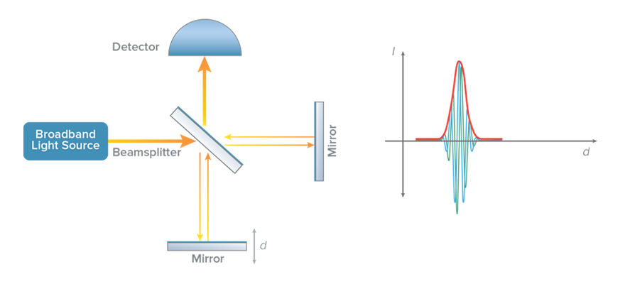
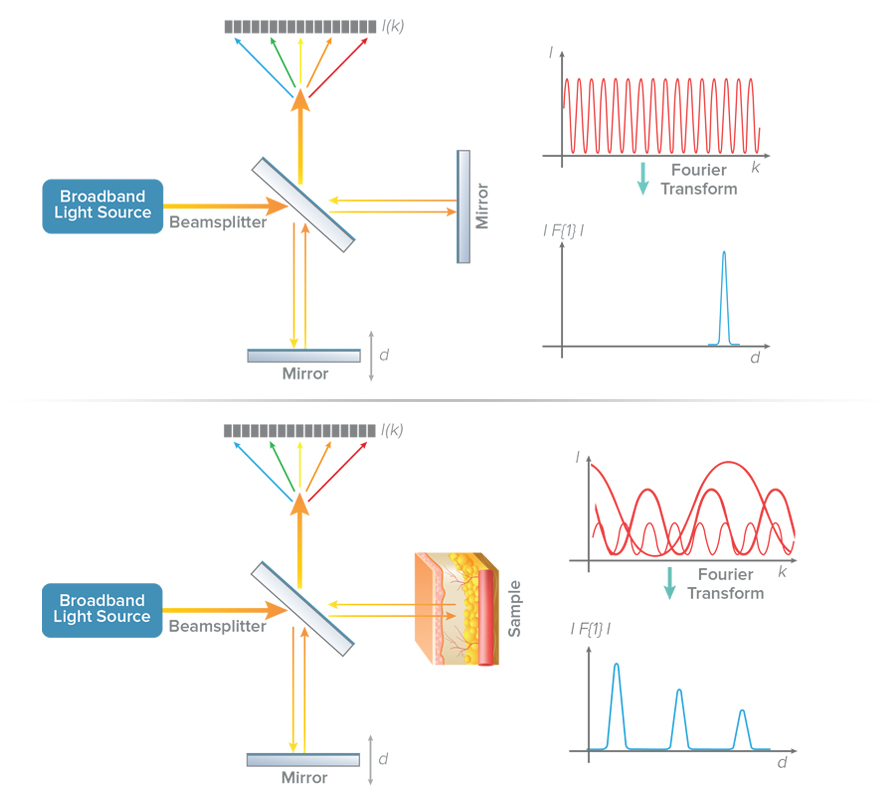
In a low-coherence interferometer, a light source with a broad optical bandwidth is used for illumination (see Figure 1). The light coming out of the source is split by a beam splitter into two paths called the reference and sample arms of the interferometer. The light from each arm is reflected back and combined at the detector. An interference effect (fast modulations in intensity) are seen at the detector only if the time travelled by light in the reference and sample arms is nearly equal. Thus the presence of interference serves as a relative measure of distance travelled by light.
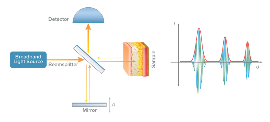
Optical coherence tomography leverages this concept by replacing the mirror in the sample arm with the sample to be imaged (Figure 2). The reference arm is then scanned in a controlled manner and the resulting light intensity is recorded on the detector. The rapid modulation interference pattern occurs when the mirror is nearly equidistant to one of the reflecting structures in the sample, and can be processed to register the presence of that structure. The distance between two mirror locations where interference occurs corresponds to the optical distance between two reflecting structures of the sample in the path of the beam. Even though the light beam passes through different structures in the sample, the low-coherence interferometry described above helps to distinguish the amount of reflection from each unique structure in the path of the beam. In doing the so, the material scattering, and hence structure, can be measured as a function of depth.
Exploring the transverse or x-y localization of the sample structure is simpler. The broadband light source beam that is used in OCT is focused to a small spot (on the order of a few micrometers) and scanned over the sample. By mapping the sample in x and y with a scanning arm while collecting depth information using interferometry, a complete 3D picture of the sample can be constructed.
Fourier-Domain OCT
Fourier-domain OCT (FD-OCT) provides an even more efficient way to implement the low-coherence interferometry described above. Instead of recording intensity at different locations of the reference mirror, the intensity is recorded as a function of the wavelengths or frequencies of the light. The intensity modulations when measured as a function of frequency are called spectral interference. The rate of variation of intensity over different frequencies is indicative of the location of the different reflecting layers in the samples. It can be shown that a Fourier transform of spectral interference data provides information equivalent to that which would be obtained by moving the reference mirror (Figure 3).
There are two common methods of measuring spectral interference in OCT: spectral-domain and swept-source. In spectral-domain OCT (SD-OCT), a broadband light source delivers many wavelengths to the sample, and all are measured simultaneously using a spectrometer as the detector. In swept-source OCT (SS-OCT), the light source is swept through a range of wavelengths and the temporal output of the detector is converted to spectral interference.
Fourier-domain OCT allows for much faster imaging than scanning of the sample arm mirror in the interferometer, as all the back reflections from the sample are being measured simultaneously. This speed increment introduced by Fourier-domain OCT has opened a whole new arena of applications for the technology. Live video, in-vivo OCT imaging can be easily obtained using commercial systems, allowing it to be used for process monitoring and guided surgery.
Key parameters for OCT Systems
Resolution
 The axial and transverse resolution of an OCT system are independent. The axial (depth) resolution is related to the bandwidth, or the coherence length, of the source. For a Gaussian spectrum, the axial resolution (λc) is given by:
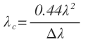
where λ is the central wavelength and Δλ is the bandwidth of the source. It should be noted that this is the spectrum measured at the detector and may differ from the spectrum of the source, due to the response of optical components and the detector itself. The above equation holds only for Gaussian spectra. For a spectrum of arbitrary shape, the axial spread function should be estimated to understand the achievable resolution and any artifacts like side lobes. Plots of the axial resolution equation for three different central wavelengths is found in figure 5, showing how axial resolution is affected by bandwidth of the source for different common operating bands in the near infrared.
Imaging depth
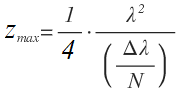
The imaging depth of OCT is primarily limited by the depth of penetration of the light source in the sample. Additionally, in Fourier-domain OCT, the depth is limited by the finite number of pixels and optical resolution of the spectrometer. As previously mentioned, the image in FD-OCT is obtained after Fourier transformation of the spectral interference data. The total length or depth after Fourier transform is limited by the sampling rate of the spectral data, and is governed by the Nyquist theorem. A total bandwidth (Δλ) sampled by N pixels gives us a wavelength sampling rate of δλ = Δλ/N. Since a Fourier transform relates frequency to time, we can convert wavelength to frequency, δν = c*Δλ /λ2. The Nyquist theorem indicates that the maximum time delay in the Fourier transformed data will be tmax = 1/2* δν, and the maximum depth in the data will be zmax = c* tmax. By combining these, the maximum imaging depth achievable in FD-OCT is:
Loss of sensitivity with depth
In Fourier domain OCT, sensitivity is in theory dependent on the location of the reflector. The maximum sensitivity occurs around the zero delay difference point and decreases as we move away from the zero delay point. This loss is the result of finite pixel size and finite optical resolution of the spectrometer. It can be shown that sensitivity is related to depth by:
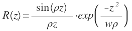
Where w is equal to δλ/Δλ and depends on the optical resolution of the spectrometer elements. The first term representing a sine function on the left hand side of the equation is the result of finite pixels in the spectrometer. The second term relates to the finite optical resolution of the spectrometer that results in ‘leakage’ of a given wavelength into multiple pixels.
Signal to Noise Ratio (SNR)
Signal to noise ratio is generally defined as the ratio of signal power to the noise level or power. Being a statistical quantity, noise power is defined by its variance. There are three main sources of noise that dominate OCT:
- The detector noise resulting mainly from thermal fluctuations in the electronics
- Shot noise due to inherent variance in the arrival and detection of photons on the detector
- Relative intensity noise (RIN) in the light source
An ideal system has minimal detector and intensity noise and operates in the shot-noise domain. The performance of such a system is limited by the number of photons arriving at the detector.
Sensitivity in OCT
Sensitivity in OCT refers to the ability of the system to detect the faintest amount of back-reflection from the sample under observation. Numerically it is the attenuation in the signal that results in a signal to noise ratio (SNR) of 1 (i.e., the point at which the signal level is equal to the inherent noise of the system).
Measurement in dB
Signal to noise ratio or sensitivity is often defined in decibels (dB). In general the dB unit of a physical quantity corresponds to 10*log(Pa/Pb). When dealing with optical light measurements the power in question should be carefully considered. The light power (P) is proportional to the current output of a photodetector (I), however the electrical power is proportional to I2 hence the SNR and sensitivity measurements in OCT when considering optical power are given by 20*log(Pa/Pb). In general, while stating values in dB, clear distinction should be made if the quantity in consideration is optical or electrical power.
Speed
The speed of an OCT system depends on several factors. The first being the amount of light received on the detector. Speed is directly related to the time the system needs to accumulate enough photons for a good signal to noise ratio. . The other limitations on speed are the system parameters themselves. For a spectrometer based spectral-domain OCT system the speed of the camera sensor and electronics are usually the limiting factor. For swept-source Fourier-domain OCT the speed of the swept source laser is often the limiting speed. While SS-OCT is often chosen for its speed, advances in camera speed in recent years have begun to close that gap.
Additional Resources

If you’d like to learn more about OCT as a technology and its many applications, we encourage you to explore a few of our favourite resources in more detail. You are also welcome to visit our OCT image gallery to see the amazing images possible with OCT. If you think OCT may be the right fit for your research, clinical, or industrial application, we’d be happy to talk more about the possibilities. Contact us and mention our tutorial!
- Brezinski, Mark E. Optical coherence tomography: principles and applications. Elsevier, 2006.
- Fercher, Adolf F., et al. “Optical coherence tomography-principles and applications.” Reports on progress in physics66.2 (2003): 239.
- Swanson, Eric A., and James G. Fujimoto. “The ecosystem that powered the translation of OCT from fundamental research to clinical and commercial impact.” Biomedical optics express 8.3 (2017): 1638-1664.
